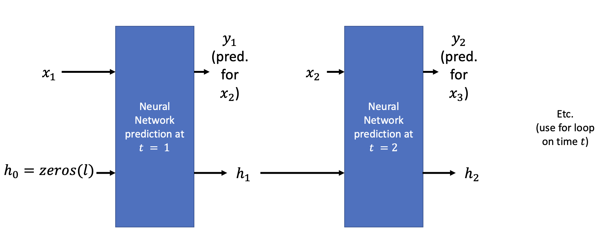
Recurrent Neural Networks

Neural Networks that receive inputs of observation $x_{t}$ at time $t$ and memory vector $h_{t}$ as outputs at time $t - 1$ , to compute a prediction $y_{t}$ for $x_{t + 1}$ and updated memory vector $h_{t + 1}$

2025-04-28_21-30-30_Recurrent Neural Networks_Diagram.png

Memory lookback

Lookback or window size refers to the number of past observations/values of a time series that is used to make a prediction

Consider the time scale of the problem to decide on appropriate lookback length:

Daily stock price prediction: Lookback length $l$ of 30 days
Hourly traffic patterns: Lookback length $l$ of 24 hours
Typically, look at the seasonality and trend (see Time series dataset#Decomposition)

Backpropagation through time

Batches of $N$ data samples per parameter update fare better than single steps:

Unfolding RNN operations over time
Run predictions on $N$ consecutive samples and keep track of loss
Perform one parameter update after $N$ samples

Vanishing gradient problem

We encounter the Vanishing gradients problem:

Each hidden state $h_{t + 1}$ is updated via a function of previous states $h_{t}$ and input $x_{t}$
During training, backpropagation through time can result in very small gradients for earlier time steps, where the weights are then updated
This is problematic as RNNs are designed to handle time series data, which can exhibit long-term dependencies
This is even more problematic if the RNN uses activation functions that saturate such as Sigmoid function or tanh function due to repeated multiplication of small derivatives and weights
As a result, weights associated with long-term dependencies update very slowly or not at all
The solution is to use specialised architectures such as Long Short-Term Memory and Gated Recurrent Units

Long Short-Term Memory and Gated Recurrent Units models work by creating more sophisticated RNN units with internal mechanisms (gates) to control the flow of information and regulate the state updates, explicitly managing what to remember and what to forget.

This decouples the task of prediction ( $x_{t + 1}$ ) from the task of memory management ( $h_{t + 1}$ ).

LSTMs vs GRUs

LSTMs > GRUs	LSTMs < GRUs
Designed to maintain and propagate info over longer time lags than GRUs, hence better suited for tasks that require network to retain info for longer periods	Fewer parameters, hence faster to train and less prone to overfitting; more computationally efficient
More parameters, hence more expressive and better able to model complex nonlinear functions	Have a simpler structure than LSTMs, hence easier to implement and understand
Can handle input sequences of variable lengths more effectively, given they have an explicit memory cell to store info over multiple timesteps	More effective in handling sequences with a lot of noise or missing data as they are able to adapt to changes
	Better suited for prioritisiation of recently observed due to the gating mechanism

Autoregressive RNNs

A type of RNN (often used in decoders) where the prediction $y_{t}$ from the current time step is used as the input $x_{t + 1}$ for the next time step

In autoregressive RNNs, the model generates sequences by feeding its own outputs back as inputs.

The encoder reads an input sequence (e.g., a French sentence, a user's question) and produces a context vector (Se).

Then, the decoder:

Uses Se as its initial hidden state $h_{0}$ and a special "start-of-sequence" token as the first input $x_{1}$ e.g. <s>
Predicts the first output word $y_{1}$
Uses $y_{1}$ as the next input $x_{2}$ to predict the second output word $y_{2}$
Continues step 3 until a special "end-of-sequence" token e.g. </s> token is generated or maximum length is reached

Autoregressive models can be harder to train because errors can accumulate. If a model makes a bad prediction early on, the incorrect prediction that is fed back in can lead to future errors - exposure bias.