Neural Networks

Definitions

NNs are computing systems inspired by the biological neural networks that constitute human brains.

They are based on a collection of connected notes called artificial neurons.

Each connection, akin to synapses in a biological brain, can transmit a signal to other neurons, therefore processing any information given as inputs to produce a final signal as output.

Training neural networks can be done with algorithms such as Backpropagation.

Simple Neural Net

__init__ method listing trainable parameters, i.e a weight vector $W = (w_{1}, w_{2})$ with 2 elements and a single scalar bias value $b$
forward method to formulate predictions for any set of given inputs $y_{i} = w_{1} s_{i} + w_{2} d_{i} + b$
Adding a loss function: Reuse the MSE
The NN could operate with any number of inputs $N_{x}$ and outputs $N_{y}$ by representing:
1. $W$ as a $N_{x} \times N_{y}$ matrix
2. $B$ as a $N_{y}$ vector

class SimpleNeuralNet():
	def __init__(self, W, b):
		self.W = W
		self.b = b
		# Add loss
		self.loss = float("Inf")
	def forward(self, x):
		Z = np.matmul(x, self.W)
		pred = Z + self.b
		return pred
	def MSE_loss(self, inputs, outputs):
		outputs_re = outputs.reshape(-1, 1)
		pred = self.forward(inputs)
		losses = (pred - outputs_re) ** 2
		self.loss = np.sum(losses) / output.shape[0]
		return self.loss

simple_nn = SimpleNeuralNet(W = np.array([], []), b = np.ones(shape = (1,1)))

Shallow Neural Net

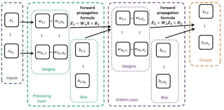
2025-03-04_16-23-49_Neural Networks_Scaling up with more layers.png

It will include two processing layers of $W X + b$ :

First layer will receive inputs with dimensionality $n_{x}$ and produce outputs with dimensionality $n_{h}$ .
Second layer called the hidden layer will receive inputs from previous layer (of the dimensionality $n_{h}$ in this case) and produce outputs with dimensionality of outputs in our dataset $n_{y}$
Hence, matrix $W$ is 2D $n_{x} \times n_{y}$ and $b$ is 1D $n_{y}$

class ShallowNeuralNet():

    def __init__(self, n_x, n_h, n_y):
        # Network dimensions
        self.n_x = n_x
        self.n_h = n_h
        self.n_y = n_y
        
        # Weights and biases matrices
        self.W1 = np.random.randn(n_x, n_h)*0.1
        self.b1 = np.random.randn(1, n_h)*0.1
        self.W2 = np.random.randn(n_h, n_y)*0.1
        self.b2 = np.random.randn(1, n_y)*0.1
        
        # Loss, initialized as infinity before first calculation is made
        self.loss = float("Inf")

    def forward(self, inputs):
        # Wx + b operation for the first layer
        Z1 = np.matmul(inputs, self.W1)
        Z1_b = Z1 + self.b1
        
        # Wx + b operation for the second layer
        Z2 = np.matmul(Z1_b, self.W2)
        Z2_b = Z2 + self.b2
        return Z2_b

    def MSE_loss(self, inputs, outputs):
        # MSE loss function as before
        outputs_re = outputs.reshape(-1, 1)
        pred = self.forward(inputs)
        losses = (pred - outputs_re)**2
        self.loss = np.sum(losses)/outputs.shape[0]
        return self.loss

We now need a training procedure since the weights and biases are currently randomly generated (See Backpropagation).

Training Procedure

Backward Method - performs calculation of gradients in matrix form and parameter adjustments using GD update rules
Forward Method - repeats backward method, reusing GD for-loop function until a maximal number of iterations is reached, or convergence is seen

i.e. the procedure:

Forward pass on dataset samples
Compute errors and loss function
Use new loss value to compute gradients
Adjust parameters with Backpropagation
Repeat until convergence or max number of iterations

def train(self, inputs, outputs, N_max = 1000, alpha = 1e-5, delta = 1e-5, display = True):
  # List of losses, starts with the current loss
  self.losses_list = [self.loss]
  # Repeat iterations
  for iteration_number in range(1, N_max + 1):
    # Backpropagate
    self.backward(inputs, outputs, alpha)
    new_loss = self.loss
    # Update losses list
    self.losses_list.append(new_loss)
    # Display
    if(display):
      print("Iteration {} - Loss = {}".format(iteration_number, new_loss))
    # Check for delta value and early stop criterion
    difference = abs(self.losses_list[-1] - self.losses_list[-2])
    if(difference < delta):
      if(display):
        print("Stopping early - loss evolution was less than delta.")
      break
    else:
      # Else on for loop will execute if break did not trigger
      if(display):
        print("Stopping - Maximal number of iterations reached.")

def show_losses_over_training(self):
  # Initialize matplotlib
  fig, axs = plt.subplots(1, 2, figsize = (15, 5))
  axs[0].plot(list(range(len(self.losses_list))), self.losses_list)
  axs[0].set_xlabel("Iteration number")
  axs[0].set_ylabel("Loss")
  axs[1].plot(list(range(len(self.losses_list))), self.losses_list)
  axs[1].set_xlabel("Iteration number")
  axs[1].set_ylabel("Loss (in logarithmic scale)")
  axs[1].set_yscale("log")
  # Display
  plt.show()

Symmetry

Initialising all parameters as identical constants (e.g. all zeros) is bad because of the tendency of all neurons to have the same weights and processes.

The lack of diversity leads to a lack of generalisation which prevents the NN from learning complex patterns.

This happens because all weights and baises had the same starting point. The backward process then updated the parameters identically and they end up keeping the same values over the course of training. Hence, we need random initialisation.

Symmetrical neural networks are vulnerable to Adversarial attacks

Model design

Constant initialisation is important to consider as it may lead to issues such as Vanishing gradients. Instead of zero/same constant initialisation, we need to use random starting values, or variants such as Xavier initialisation.

Selecting a proper learning rate is also important to tackle Exploding gradients.

Also, if our model only consists of two linear layers (as seen above), the boundary for our models is also linear in $x_{1}$ and $x_{2}$ , and we cannot model more complex behaviour. Hence, we need to rely on Activation functions

Introducing non-linearity

Adding sigmoid operations after each linear operation in the forward method:

def forward(self, inputs):
  # Wx + b operation for the first layer
  Z1 = np.matmul(inputs, self.W1)
  Z1_b = Z1 + self.b1
  A1 = self.sigmoid(Z1_b)
  # Wx + b operation for the second layer
  Z2 = np.matmul(A1, self.W2)
  Z2_b = Z2 + self.b2
  y_pred = self.sigmoid(Z2_b)
  return y_pred

This requires the backward propagation to be updated.

Inputs X
Linear #1
Z₁ = W₁X + b₁
Sigmoid
A₁ = s(Z₁)
Linear #2
Z₂ = W₂X + b₂
Sigmoid
A₂ = s(Z₂)
Cross Entropy Loss
L(A₂, Y)

LinReg + Sigmoid = LogReg, so LinReg Layer + Sigmoid = LogReg Layer?

Throwing formulas around:

\begin{aligned} Z_{1} & = W_{1} X + b_{1} \\ A_{1} & = s (Z_{1}) \\ Z_{2} & = W_{2} A_{1} + b_{2} \\ A_{2} & = s (Z_{2}) \\ L & = \frac{- 1}{N} \sum_{i}^{N} Y \ln (A_{2}) + (1 - Y) \ln (1 - A_{2}) \\ \frac{\partial L}{\partial A_{2}} & = - \frac{Y}{A_{2}} + \frac{1 - Y}{1 - A_{2}} \end{aligned}

\begin{aligned} A_{2} & = s (Z_{2}) \\ s^{'} (X) & = s (X) (1 - s (X)) \\ \frac{\partial L}{\partial Z_{2}} & = \frac{\partial L}{\partial A_{2}} \frac{\partial A_{2}}{\partial Z_{2}} = \frac{\partial L}{\partial A_{2}} A_{2} (1 - A_{2}) \end{aligned}

\begin{aligned} Z_{2} & = W_{2} A_{1} + b_{2} \\ \frac{\partial L}{\partial W_{2}} & = \frac{\partial L}{\partial Z_{2}} \frac{\partial Z_{2}}{\partial W_{2}} = \frac{\partial L}{\partial Z_{2}} A_{1} \\ \frac{\partial L}{\partial b_{2}} & = \frac{\partial L}{\partial Z_{2}} \frac{\partial Z_{2}}{\partial b_{2}} = \frac{\partial L}{\partial Z_{2}} \\ A_{1} & = s (Z_{1}) \\ \frac{\partial L}{\partial A_{1}} & = \frac{\partial L}{\partial Z_{2}} \frac{\partial Z_{2}}{\partial A_{1}} = \frac{\partial L}{\partial Z_{2}} W_{2} \\ \frac{\partial L}{\partial Z_{1}} & = \frac{\partial L}{\partial A_{1}} \frac{\partial A_{1}}{\partial Z_{1}} = \frac{\partial L}{\partial A_{1}} A_{1} (1 - A_{1}) \end{aligned}

\begin{aligned} Z_{1} & = W_{1} X + b_{1} \\ \frac{\partial L}{\partial W_{1}} & = \frac{\partial L}{\partial Z_{1}} \frac{\partial Z_{1}}{\partial W_{1}} = \frac{\partial L}{\partial Z_{1}} X \\ \frac{\partial L}{\partial b_{1}} & = \frac{\partial L}{\partial Z_{1}} \frac{\partial Z_{1}}{\partial b_{1}} = \frac{\partial L}{\partial Z_{1}} \end{aligned}

Updating our backward method:

def backward(self, inputs, outputs, alpha = 1e-5):
    # Get the number of samples in dataset
    m = inputs.shape[0]

    # Forward propagate
    Z1 = np.matmul(inputs, self.W1)
    Z1_b = Z1 + self.b1
    A1 = self.sigmoid(Z1_b)
    Z2 = np.matmul(A1, self.W2)
    Z2_b = Z2 + self.b2
    A2 = self.sigmoid(Z2_b)

    # Compute error term
    dL_dA2 = -outputs/A2 + (1 - outputs)/(1 - A2)
    dL_dZ2 = dL_dA2*A2*(1 - A2)
    dL_dA1 = np.dot(dL_dZ2, self.W2.T)
    dL_dZ1 = dL_dA1*A1*(1 - A1)

    # Gradient descent update rules
    self.W2 -= (1/m)*alpha*np.dot(A1.T, dL_dZ2)
    self.W1 -= (1/m)*alpha*np.dot(inputs.T, dL_dZ1)
    self.b2 -= (1/m)*alpha*np.sum(dL_dZ2, axis = 0, keepdims = True)
    self.b1 -= (1/m)*alpha*np.sum(dL_dZ1, axis = 0, keepdims = True)

    # Update Loss
    self.CE_loss(inputs, outputs)

We use Activation functions to introduce non-linearity into our models. Sigmoid and tanh functions are often used, but both often lead to vanishing gradients.

Hence, we can use ReLU function or Leaky ReLU function due to their computational efficiencies and prevention of saturation

Improving gradient descent

We can improve gradient descent further (see Gradient Descent#Improving gradient descent) by introducing Momentum, Gradient-based learning rate control and Learning rate decay through different optimisation algorithms

Examples of optimisers

AdaGrad
RMSProp
Adam optimiser
AdaBound - Adam + AdaGrad
AMSGrad - Improved Adam
Lookahead - Adam + Momentum

Improving computation rate

We can perform parameter training updates with smaller batches of the dataset rather than the entire dataset per iteration by utilising Stochastic Gradient Descent, ideally mini-batch.

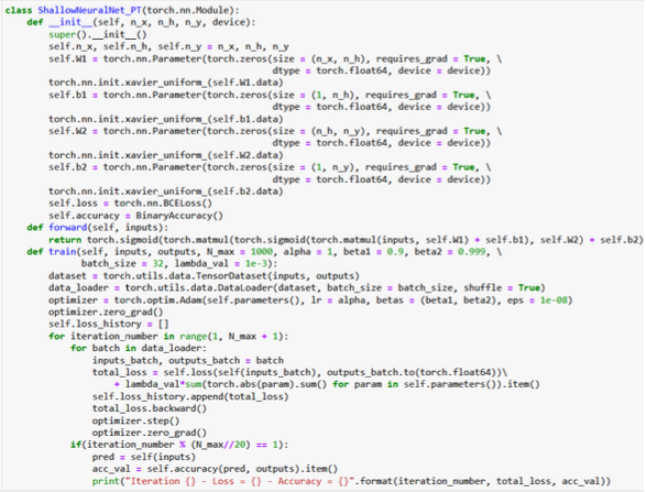
Good Practices

Additional performance metrics

Low loss does not mean successful training, because we have only minimised it. We should instead use more interpretable performance metrics

For instance, using accuracy:

def accuracy(self, inputs, outputs):
    # Calculate accuracy for given inputs and ouputs
    pred = [int(val >= 0.5) for val in self.forward(inputs)]
    acc = sum([int(val1 == val2[0]) for val1, val2 in zip(pred, outputs)])/outputs.shape[0]
    return acc

def train(self, inputs, outputs, N_max = 1000, alpha = 1e-5, beta1 = 0.9, beta2 = 0.999, \
          delta = 1e-5, batch_size = 100, display = True):
    # Get number of samples
    M = inputs.shape[0]

    # List of losses, starts with the current loss
    self.losses_list = [self.CE_loss(inputs, outputs)]
    self.accuracies_list = [self.accuracy(inputs, outputs)]

Train-test-validation split

We are not here to minimise the training loss function (or maximise accuracy) but to generalise well on unseen data. So expanding on Train and test split, we introduce a validation dataset.

This will help us access the performance of the model and how well it would generalise.

Spotting Overfitting and Underfitting
Choosing best Hyperparameters

Implementing early stop

In general,

Model will start by underfitting the data, which is normal.
After a few rounds of training models will (hopefully) achieve good generalization.
Then, if training is pursued, the model will often attempt to minimize loss at all costs, often sacrificing generalisation in the process, and overfitting.

We should try and stop the training when the model starts losing it generalization capabilities and starts overfitting, when:

Validation loss is minimal
Validation and training curves start going in opposite ways

Early stopping can be defined by interrupting training when:

A sufficiently high accuracy has been obtained (e.g. 98%)
Accuracy is no longer increasing as the change between two consecutive iterations of accuracy falls below a threshold $ϵ$

Saver and Loader functions

Since we will often stop training after it is too late (after it loses generalisation capabilities), we should save model parameters every $K$ iterations

def save(self, path_to_file, iter_num = "final"):
    # Display
    folder = path_to_file + "/" + iter_num + "/"
    print("Saving model to", folder)

    # Check if directory exists
    if(not os.path.exists(folder)):
        os.mkdir(folder)

    # Dump
    with open(folder + "W1.pkl", 'wb') as f:
        pickle.dump(self.W1, f)
        f.close()
    with open(folder + "W2.pkl", 'wb') as f:
        pickle.dump(self.W2, f)
        f.close()
    with open(folder + "b1.pkl", 'wb') as f:
        pickle.dump(self.b1, f)
        f.close()
    with open(folder + "b2.pkl", 'wb') as f:
        pickle.dump(self.b2, f)
        f.close()

# Save model
self.save("./save", iter_num = str(iteration_number))

After training, load the model parameters ( $W_{1}, W_{2}, b_{1}, b_{2}$ ) that correspond to the best iteration for generalisation, e.g. by manually analysing training curves

Saving is also used to ensure reproducibility of results and preventing data loss.

2025-03-06_00-54-04_Neural Networks_ShallowNeuralNet_PT.png

Dense Neural Networks

A neural network with more than two hidden layers

Good practices

Size of layers should progressively decrease by a factor of at least 2 e.g. $[80, 40, 20, 10]$
Create building blocks for modularity

class DenseReLU(torch.nn.Module):
    def __init__(self, n_x, n_y):
        super().__init__()
        # Define Linear layer using the nn.Linear()
        self.fc = torch.nn.Linear(n_x, n_y)

    def forward(self, x):
        # Wx + b operation
        # Using ReLU operation as activation after
        return torch.relu(self.fc(x))

class DenseNoReLU(torch.nn.Module):
    def __init__(self, n_x, n_y):
        super().__init__()
        # Define Linear layer using the nn.Linear()
        self.fc = torch.nn.Linear(n_x, n_y)

    def forward(self, x):
        # Wx + b operation
        # No activation function
        return self.fc(x)

Assemble the building blocks into a large Deep NN object

class DeepNeuralNet(torch.nn.Module):
    def __init__(self, n_x, n_h, n_y):
        super().__init__()
        # Define three Dense + ReLU Layers,
        # followed by one Dense + Softmax Layer
        self.layer1 = DenseReLU(n_x, n_h[0])
        self.layer2 = DenseReLU(n_h[0], n_h[1])
        self.layer3 = DenseReLU(n_h[1], n_h[2])
        self.layer4 = DenseNoReLU(n_h[2], n_y)

        # Combine all four layers
        self.combined_layers = torch.nn.Sequential(self.layer1,
											       self.layer2,
                                                   self.layer3,
	                                               self.layer4)

    def forward(self, x):
        # Flatten images (transform them from 28x28
        # 2D matrices to 784 1D vectors)
        x = x.view(x.size(0), -1)
        # Pass through all four layers
        out = self.combined_layers(x)
        return out

# Initialize the model and optimizer
model = DeepNeuralNet(n_x=784, n_h=[80, 40, 20], n_y=10).to(device)
optimizer = torch.optim.Adam(model.parameters(), lr=1e-3)

Deeper networks may be prone to overfitting if the network is too deep.

Conversely, shallower networks may be easier to train and require less data but may not be able to learn as complex patterns.