Convolution

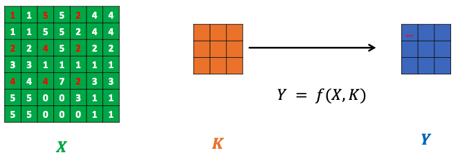
Mathematical operation: applies a small matrix called a convolution kernel or filter $K$ over a given image $X$ , element-wise multiplying each overlapping set of values with the kernel and then summing the results

Y = f (X, K)

Each output represents the sum of the product of the input and the pixel.

Used in Computer vision. For instance $Y = f (X, K)$ produces an image $Y$ of size $h^{'} \times w^{'}$ , with $h^{'} = h - k + 1$ and $w^{'} = w - k + 1$

Types of kernels

Choosing the right kernel size for convolution:

Larger kernel preferred for information distributed more globally (zoomed-in)
Smaller kernel preferred for information distributed more locally (zoomed-out)

Conv2d

def convolution_batch_torch_conv2d(images, kernel, stride = 1, padding = 0):
    # Convert kernel to PyTorch tensor, if needed
    kernel = torch.from_numpy(kernel)
    kernel = kernel.view(1, 1, kernel.shape[0], kernel.shape[1])
    kernel = kernel.float()

    # Flip the kernel (optional)
    kernel = torch.flip(torch.flip(kernel, [2]), [3])

    # Create a convolutional layer
    conv = torch.nn.Conv2d(in_channels = images.shape[1], \
                           out_channels = 1, \
                           kernel_size = kernel.shape[2:], \
                           stride = stride, \
                           padding = padding)

    # Assign the kernel to the layer
    conv.weight = torch.nn.Parameter(kernel)
    conv.bias = torch.nn.Parameter(torch.tensor([0.0]))

    # Perform convolution
    output = conv(images)

    return output

Y_{i, j} = \frac{1}{k^{2}} \sum_{m = 1}^{k} \sum_{n = 1}^{k} X_{i + m - 1, j + n - 1} K_{m, n} + b

Formatted as a 4D tensor of size $N_{s} \times c \times h \times w$ , where:

$N_{s}$ the number of samples/images in batch of data $X$ ,
$c$ , the number of channels in images of batch $X$ (e.g. greyscale = 1, RGB = 3),
$h$ , the height for images batch of data $X$ ,
$w$ , the width for images batch of data $X$ .

For RGB (not grayscale images), follow #Higher dimension convolution.

Chaining convolutions

nn.Conv2d(1, 32, kernel_size = 3, stride = 1, padding = 1)

The first two integer values correspond to the number of channels of input images X and the number of channels in kernel.

The convolution layer below then expects grayscale images X with only one channel and will produce images Y with 32 channels.

This image $Y$ with 32 channels can be visualised as 32 different convolution operations on 32 different kernels.

These filters are initialised (see Constant initialisation), and the Convolutional Neural Networks will learn the best filters on its own.

nn.Conv2d(32, 64, kernel_size=3, stride=1, padding=1)

By stacking multiple convolutional layers, the network can learn hierarchical features, where lower layers detect simple patterns and higher layers detect more complex structures.

Padding

Convolution produces a new image $Y$ whose size and resolution has been reduced, as it sums several pixels together but only produces one pixel. Larger kernels result with even smaller outputs.

Hence, we have to pad the image - add extra pixels on the outer part of the original image. This artificially increases the size of the original mimage $X$ such that the output image $Y$ matches in size with $X$ .

Valid padding

By default, with no padding applied to the input data. Convolution is thus only performed on the valid parts of input, with the output size being smaller than the input size.

Same padding

We add a padding size $p$ of zeros so that $Y$ is same-sized as $X$

When using a padding with size $p$ , we need to redefine $h^{'}$ and $w^{'}$ as:

$h^{'} = h + 2 p - k + 1$
$w^{'} = w + 2 p - k + 1$

Thus, the padding size $p = \frac{k - 1}{2}$ if we want to ensure $Y$ has the same dimensions as $X$ .

Interpolation padding

Similar to same padding, but we use the value of the closest pixel instead of zeros. This supports zooming into the original image, which means we can resize the image and then apply interpolation techniques before convolution such that the output $Y$ has the same size as $X$ .

2025-03-06_01-39-59_Convolution_Interpolation padding.png

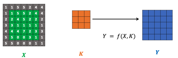
image = np.pad(image, ((padding, padding), (padding, padding)), 'constant')

Stride

Controls the movement or step size of the convolution filter as it slides over the input image

Larger stride results in a smaller output feature map, and the converse is true.

Stride can help reduce the spatial dimensions of the feature map, reducing the number of parameters and computation.

A stride of 2 means we are sliding to every other pixel.

Dilation

Spacing between values of original image multiplying the kernel. By default $d = 1$

For $d > 1$ , the pixel values are spread apart by $d$ pixels

2025-03-06_01-53-08_Convolution_Dilation example.png

Convolution formula

Given a 3D tensor $X$ of size $h \times w \times c$ , of height $h$ , weight $w$ and number of channels $c$
A convolution kernel $K$ of size $k \times k$
A padding of size $p$ , a stride of size $s$ , a dilation of size $d$

The resulting image $Y$ will have a size $h^{'} \times w^{'} \times c$ , where:

\begin{aligned} h^{'} & = ⌊ \frac{h + 2 p - d (k - 1) - 1}{s} + 1 ⌋ \\ w^{'} & = ⌊ \frac{w + 2 p - d (k - 1) - 1}{s} + 1 ⌋ \end{aligned}

& Floor function used in case division result has to be an integer

Higher dimension convolution

With a 2D kernel:

For pixels $Y_{i, j, l}$ ,

\begin{aligned} \forall i \in [1, h^{'}], j \in [1, w^{'}], \forall l \in [1, 3] : \\ Y_{i, j, l} = \frac{1}{k^{2}} \sum_{m = 1}^{k} \sum_{n = 1}^{k} X_{i + m - 1, j + n - 1, l} K_{m, n} + b \end{aligned}

This preserves the original number of channels of original image $X$ , producing new RGB image $Y$

For a kernel as a tensor with its own number of channels $k_{d} \neq 1$ :

For pixels $Y_{i, j, l}$ calculated using the convolution operation on each channel separately,

\begin{aligned} \forall i \in [1, h^{'}], j \in [1, w^{'}], \forall l \in [1, k_{d}] : \\ Y_{i, j, l} = \sum_{m = 1}^{k} \sum_{n = 1}^{k} \sum_{l^{'} = 1}^{3} X_{i + m - 1, j + n - 1, l^{'}} K_{m, n, l} + b \end{aligned}

This produces a new image $Y$ , with number of channels matching kernel $K$ i.e. $h^{'} \times w^{'} \times k_{d}$